Easy 2-Factor ANOVA in R

The CGPfunctions provides a super-fast method to visualize the complete results of a two-factor ANOVA.

Last updated on June 26, 2023 4 min read Util

Libraries


require(tidyverse)
require(CGPfunctions)
require(skimr)
require(Hmisc) # %nin%
require(cowplot)

Data

You can download the data using this link

data <- read.csv(file = path)

Data Wrangling

data %>% head()
data %>% skimr::skim()

data <- janitor::clean_names(data)

data <- 
   data %>%
   filter(gender %nin% c("","Other"),
          education_level %nin% c("","Other")) %>% 
   mutate(gender = factor(gender,levels = c("Male","Female")),
                education_level = factor(education_level, 
                                         levels  = data$education_level[data$education_level %nin%c("","Other")] %>% unique()))

data %>% count(education_level) # There's a PhD coded as phD
#data[which(data$education_level == "phD"),"education_level"] = "PhD"
#data[which(data$education_level == "Bachelor's Degree"),"education_level"] = "Bachelor's"
#data[which(data$education_level == "Master's Degree"),"education_level"] = "Master's"

# education_level should be ordered
data$education_level <- factor(data$education_level,levels = c("High School","Bachelor's","Master's","PhD"))

Descriptive plots

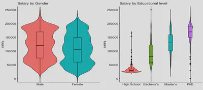
Let’s graph the variables we are interested in

a1 <- 
   ggpubr::ggviolin(data %>% filter(gender != "Other"), 
               y = "salary", x = "gender",
               add = "boxplot",
               fill = "gender")+
   coord_cartesian(ylim = c(0,250000)) +
   xlab("")+
   theme(legend.position = "none")+
   ggtitle("Salary by Gender")

a2 <- 
   ggpubr::ggviolin(data %>% filter(gender != "Other"), 
               y = "salary", x = "education_level",
               add = "boxplot",
               fill = "education_level")+
   coord_cartesian(ylim = c(0,250000)) +
   xlab("")+
   theme(legend.position = "none")+
   ggtitle("Salary by Educational level")

cowplot::plot_grid(a1,a2)

ANOVA 2WAY

We are going to proceed with the two way ANOVA. I want to remember that a good practice would be to check the assumptions before directly jumping into the analysis. However, the objective of this post is to provide a preview of the function and its output.

CGPfunctions::Plot2WayANOVA(dataframe = data,
                            formula = salary ~ education_level*gender,
                            errorbar.display = "SEM",
                            mean.label = T)

The function returns four main outputs:

Main result of the ANOVA
Descriptive table of disaggregated means with confidence intervals and errors
Posthoc analysis
Interaction plot

Anova Results

The object can be saved for easier access to its elements. For example, to better visualize the overall ANOVA table, you can access it through the command: o1$ANOVATable.

print(o1$ANOVATable[c("term","df","statistic","p.value","etasq","cohens.f")])

According to the results, we can see that both the effects of the two variables and the interaction are significant in the model.

#Descriptive table of disaggregated means with confidence intervals and errors
o1$MeansTable

post-hoc analyses

An important output is the post-hoc analysis. We can observe the main effects within each factor and the comparisons between the interaction of the levels. We can change the approach of these analyses within the parameter of the function posthoc.method

o1$PosthocTable


# Posthoc multiple comparisons of means: Scheffe Test 
#    95% family-wise confidence level
#
#$education_level
#                            diff    lwr.ci    upr.ci   pval    
#Bachelor's-High School  60667.30  53067.99  68266.60 <2e-16 ***
#Master's-High School    95662.77  87769.20 103556.34 <2e-16 ***
#PhD-High School        131235.85 123078.73 139392.96 <2e-16 ***
#Master's-Bachelor's     34995.48  30622.17  39368.78 <2e-16 ***
#PhD-Bachelor's          70568.55  65735.76  75401.34 <2e-16 ***
#PhD-Master's            35573.07  30289.62  40856.52 <2e-16 ***
#
#$gender
#                 diff    lwr.ci    upr.ci   pval    
#Female-Male -11218.79 -14865.24 -7572.353 <2e-16 ***
#
#$`education_level:gender`
#                                            diff     lwr.ci       upr.ci    pval    
#Bachelor's:Male-High School:Male       59591.017   48145.24   71036.7985 < 2e-16 ***
#Master's:Male-High School:Male        100679.841   88564.22  112795.4623 < 2e-16 ***
#PhD:Male-High School:Male             129330.320  117324.48  141336.1620 < 2e-16 ***
#High School:Female-High School:Male    -8624.704  -22998.23    5748.8221  0.6516    
#Bachelor's:Female-High School:Male     49784.468   38066.84   61502.0935 < 2e-16 ***
#Master's:Female-High School:Male       83313.791   71501.15   95126.4271 < 2e-16 ***
#PhD:Female-High School:Male           120885.541  108106.75  133664.3283 < 2e-16 ***
#Master's:Male-Bachelor's:Male          41088.824   34770.45   47407.2020 < 2e-16 ***
#PhD:Male-Bachelor's:Male               69739.303   63634.07   75844.5360 < 2e-16 ***
#High School:Female-Bachelor's:Male    -68215.721  -78202.30  -58229.1365 < 2e-16 ***
#Bachelor's:Female-Bachelor's:Male      -9806.549  -15323.47   -4289.6325 1.8e-07 ***
#Master's:Female-Bachelor's:Male        23722.774   18006.83   29438.7164 < 2e-16 ***
#PhD:Female-Bachelor's:Male             61294.524   53782.46   68806.5828 < 2e-16 ***
#PhD:Male-Master's:Male                 28650.479   21366.51   35934.4503 < 2e-16 ***
#High School:Female-Master's:Male     -109304.545 -120052.30  -98556.7899 < 2e-16 ***
#Bachelor's:Female-Master's:Male       -50895.373  -57693.81  -44096.9367 < 2e-16 ***
#Master's:Female-Master's:Male         -17366.050  -24326.97  -10405.1330 4.9e-16 ***
#PhD:Female-Master's:Male               20205.700   11707.85   28703.5466 2.1e-14 ***
#High School:Female-PhD:Male          -137955.023 -148578.87 -127331.1724 < 2e-16 ***
#Bachelor's:Female-PhD:Male            -79545.851  -86146.66  -72945.0403 < 2e-16 ***
#Master's:Female-PhD:Male              -46016.529  -52784.57  -39248.4906 < 2e-16 ***
#PhD:Female-PhD:Male                    -8444.779  -16785.36    -104.1929  0.0442 *  
#Bachelor's:Female-High School:Female   58409.172   48112.15   68706.1954 < 2e-16 ***
#Master's:Female-High School:Female     91938.494   81533.48  102343.5091 < 2e-16 ***
#PhD:Female-High School:Female         129510.245  118020.10  141000.3864 < 2e-16 ***
#Master's:Female-Bachelor's:Female      33529.323   27286.82   39771.8248 < 2e-16 ***
#PhD:Female-Bachelor's:Female           71101.073   63180.98   79021.1651 < 2e-16 ***
#PhD:Female-Master's:Female             37571.750   29511.76   45631.7438 < 2e-16 ***
#
#---
#Signif. codes:  0 '***' 0.001 '**' 0.01 '*' 0.05 '.' 0.1 ' ' 1
#

ANOVA plot

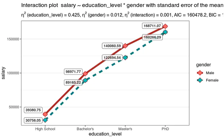
Lastly, and perhaps more illustrative, the graph of simple effects. To change the simple effect, we just need to alter the direction of the interaction within the parameter of the function.


CGPfunctions::Plot2WayANOVA(dataframe = data,
                            formula = salary ~ education_level*gender, # switch for different graph
                            errorbar.display = "SEM",
                            mean.label = T)

Additionally, the function easily provides us with the Bayesian analysis of the model and the assessment of the assumption of homoscedasticity.

o1$Bayesian_models
# 
#   model                                                    bf support                    margin_of_error
#   <chr>                                                 <dbl> <chr>                                <dbl>
# 1 education_level                                   Inf       " data support is extreme"        1.47e- 7
# 2 education_level + gender                          Inf       " data support is extreme"        1.28e- 2
# 3 education_level + gender + education_level:gender Inf       " data support is extreme"        4.45e- 2
# 4 gender                                              1.23e22 " data support is extreme"        2.05e-26

ANOVA 2way ANOVA R R for Publication