Printing and Exporting Linear Regression Models

A concise example of linear regression and its export in R for publication

Last updated on June 18, 2023 3 min read Util

Set up

#libraries

require(tidyverse)
#require(lme4)
require(jtools)
require(skimr)
require(correlation)
require(corrplot)

You can download the data in the following link: https://www.kaggle.com/datasets/hellbuoy/car-price-prediction

#import data base 
carlr <- read.csv(file = "/Users/adri/Downloads/car_price_prediction/CarPrice_Assignment.csv")
carlr %>% head()

Explore Data

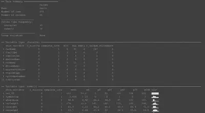
As always, it is advisable to explore the data initially. By examining the data’s surface and its coding, we can gain a better understanding of its structure and identify any errors. Additionally, this exploration may reveal relationships or analyses that were not initially considered during the data programming stage.

#first look at the data
skimr::skim(carlr)

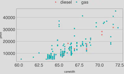
We can also use graphical representations to explore the variables of interest.

# Podemos hacer algun scatter plot de dos variables contínuas que pensemos estén relacionadas
ggpubr::ggscatter(carlr,
                  x = "carwidth", y = "price",
                  color = "fueltype")+
   jtools::theme_apa()

We can quickly examine the linear correlations between numerical variables.

Correlation table

car_cor <- correlation::correlation(data =carlr %>% select_if(is.numeric)) # podemos visualizasrlo en tabla
car_cor %>% filter(p < 0.05) # we can apply dplyr logic to the object

PRINT ________________________________

# Correlation Matrix (pearson-method)

#Parameter1       |       Parameter2 |     r |         95% CI | t(203) |         p
#---------------------------------------------------------------------------------
#car_ID           |        carheight |  0.26 | [ 0.12,  0.38] |   3.77 | 0.012*   
#car_ID           |        boreratio |  0.26 | [ 0.13,  0.38] |   3.84 | 0.010**  
#symboling        |        wheelbase | -0.53 | [-0.62, -0.43] |  -8.95 | < .001***
#symboling        |        carlength | -0.36 | [-0.47, -0.23] |  -5.46 | < .001***
#symboling        |         carwidth | -0.23 | [-0.36, -0.10] |  -3.41 | 0.042*   
#symboling        |        carheight | -0.54 | [-0.63, -0.44] |  -9.17 | < .001***
#symboling        |          peakrpm |  0.27 | [ 0.14,  0.40] |   4.05 | 0.005**  
#wheelbase        |        carlength |  0.87 | [ 0.84,  0.90] |  25.70 | < .001***
#wheelbase        |         carwidth |  0.80 | [ 0.74,  0.84] |  18.68 | < .001***
#wheelbase        |        carheight |  0.59 | [ 0.49,  0.67] |  10.40 | < .001***
#---

#p-value adjustment method: Holm (1979)
#Observations: 205

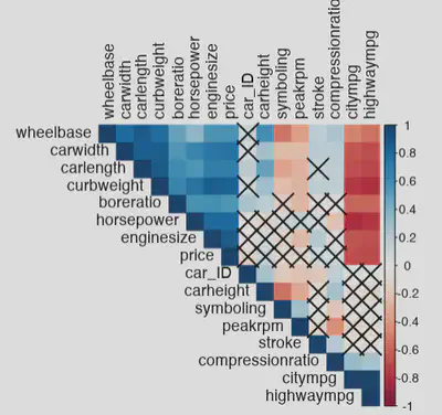
Correlation plot

Alternatively, we can create a correlation chart.


corrplot::corrplot(corr = cor(carlr %>% select_if(is.numeric)),
                   type = "upper",
                   method = "color",
                   order = "hclust",
                   #addCoef.col = 'black',
                   p.mat = car_mtest$p,
                   tl.col = "black")

Linear Regression and exportation

In practice, it is best to test the relationships we have in mind beforehand. However, in reality, exploratory analyses often lead to post-hoc models. Without delving too much into statistics, we will demonstrate how to create a simple linear regression model and export it.

# Simple prediction 
## Price ~ engine size

lm(data = carlr, 
   formula = price ~ enginesize) %>% 
   jtools::summ()

PRINT ________________________


#MODEL INFO:
#Observations: 205
#Dependent Variable: price
#Type: OLS linear regression 
#
#MODEL FIT:
#F(1,203) = 657.64, p = 0.00
#R² = 0.76
#Adj. R² = 0.76 
#
#Standard errors: OLS
#-----------------------------------------------------
#                        Est.     S.E.   t val.      p
#----------------- ---------- -------- -------- ------
#(Intercept)         -8005.45   873.22    -9.17   0.00
#enginesize            167.70     6.54    25.64   0.00
#-----------------------------------------------------

Adding more variables, creating multiple models, and comparing them

# Adding more variables and storing them in different models

modelo_1 <- lm(data = carlr,
           formula = price ~ enginesize)

modelo_2 <- lm(data = carlr,
           formula = price ~ enginesize + citympg)

modelo_3 <- lm(data = carlr,
           formula = price ~ enginesize + citympg+ curbweight+carheight)

modelo_4 <- lm(data = carlr,
           formula = price ~ enginesize + citympg+ curbweight+carheight + factor(fueltype))

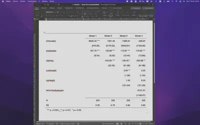
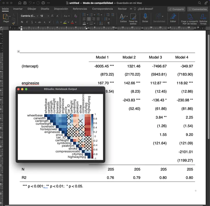
jtools::export_summs(modelo_1,modelo_2, modelo_3, modelo_4) # print as many models as you want together

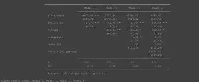
The jtools::export_sums() function includes a method to export directly to word

jtools::export_summs(modelo_1,modelo_2, modelo_3, modelo_4,
                     to.file = "word")

Linear Regression Export lm Correlation R R for Publication